
This is a continuation of my previous proof-of-concept posts on applying machine learning algorithms on microbiome data for diagnostic platform development.
Copyright Declaration
Except for the image above this declaration, and unless otherwise stated, the author asserts his copyright over this file and all files written by him containing links to this copyright declaration under the terms of the copyright laws in force in the country you are reading this work in.
This work is copyright © Ali A. Faruqi 2016. All rights reserved.
1. Introduction
In order to make medicine truly predictive, we need powerful predictive models that can handle noisy biological datasets. In order to make medicine preventive, we need to detect diseases early on. In this context, disease detection is essentially a problem of classification. Given the input data from an individual, we’d wish to classify the person’s disease status i.e., whether the individual has a disease or not. Once we truly appreciate this fact, we can work towards building better platforms with more sophisticated models that account for the subtleties and stochasticity of biological systems.
Microbiome profile is a proxy for various diseases. Using it as an input, we’d like to know the disease status of an individual. In this post, I will explore the application of some classical machine learning algorithms on microbiome data and see how well they compare to models implemented in TensorFlow that I discussed in my earlier posts, here and here.
This post is a continuation of my previous proof-of-concept posts in which I was using a microbiome dataset as input to deep-learning models in order to predict the HIV status based on a study by Lozupone et al.
2. Technical Details
A number of models exist in machine learning literature that are suitable for classification tasks. Many of these models have different parameters that are not directly learned during the training session. The optimal values of these parameters can be searched in a user-defined parameter search space and subsequently cross-validated.
For this purpose, I ran the GridSearchCV() method with a 3-fold cross-validation on 4 out of the 5 models, which required parameter tuning. I left one model out because it was fairly simple and had no complicated parameters to be searched and cross-validated. The script is called gridsearch.py.
Below are some of the models that I have used in this exploratory analysis that are available in the Python machine learning library, scikit-learn.
2A. Gaussian Naive Bayes
Gaussian Naive Bayes is one of the simplest algorithms used for classification purposes. In this model, the likelihood of the features is assumed to follow a normal distribution. The classifier is called Naive Bayes because it relies on the Bayes theorem to determine the posterior i.e., probability of belonging to a class, given the features. It’s naive in its assumption that all features are independent.
I used the GaussianNB() class from scikit-learn library with default settings.
2B. Random Forests
Random Forest classifier is a machine-learning algorithm falling under the category of ensemble learning, which takes the bagging (bootstrap aggergating) approach. Briefly, random forest, as the name suggests, consists of many (random) trees. Each tree is a classifier that is trained independently of other trees. As a classifier, the tree is developed by randomly selecting a subset of features and performing a split over a number of nodes. The result is the predictions provided by the leaf nodes of the tree. Random forest does this for multiple trees. The final predictions are obtained by averaging over the forest.
According to An Introduction to Statistical Learning: with Applications in R:
[A] natural way to reduce the variance and hence increase the prediction accuracy of a statistical learning method is to take many training sets from the population, build a separate prediction model using each training set, and average the resulting predictions… Of course, this is not practical because we generally do not have access to multiple training sets. Instead, we can bootstrap, by taking repeated samples from the (single) training data set… This is called bagging… The main difference between bagging and random forests is the choice of predictor subset size m. For instance, if a random forest is built using m = p, then this amounts simply to bagging.
Usually, for random forests, the number of predictors considered at each split is approximately equal to the square root of the total number of predictors.
I used the RandomForestClassifier() class from scikit-learn library for prediction. Based on cross-validated grid-search, I used n_estimators = 1000, which is the number of trees and set random_state = 0 as seed for the pseudo random number generator (PRNG).
2C. Gradient Tree Boosting
Like Random Forests, Gradient Tree Boosting classifier is also part of ensemble learning. Unlike Random Forests, it relies on the boosting approach. In boosting, the classifiers are trained sequentially. That is, each new tree is grown utilizing information from trees grown previously. Also, unlike the bootstrapping approach of random forest, in boosting, new decision trees are fit to the residuals of the model. So, instead of fitting the data hard by using a single large decision tree, boosting learns slowly.
According to the book, An Introduction to Statistical Learning: with Applications in R, the three main parameters to tune in boosting trees are:
- The number of trees: Boosting can overfit if number of trees is large.
- The shrinkage parameter (λ): This is also called the learn rate and controls the rate at which boosting learns. Small values of λ require large number of trees in order to have good performance.
- Number of splits on each tree (d): This is also called maximum depth of the tree and controls the complexity of the boosted ensemble.
I used GradientBoostingClassifier() class with n_estimators=1000, learning_rate=1, max_depth=10 and min_samples_split=5 based on the cross-validated grid-search. The value of random_state was set to 0, which is the seed for PRNG. Rest were default values.
2D. Support Vector Machines (SVMs)
Support Vector Machines (SVMs) are class of supervised learning algorithms that have historically been used for classification purposes. The idea has been to come up with hyper-plane or set of hyper-planes that can separate the samples in two or more classes.
I used SVC() class of scikit-learn library to apply SVM on the dataset. Based on the results of cross-validated grid search, I chose the default Radial Basis Function (RBF) kernel SVM with C=10 and gamma=0.001
2E. Multi-layer Perceptron (MLP)
The multi-layer perceptron is a type of artificial neural network that trains using backpropogation. In it’s simplest case, it can be considered as a logistic regression classifier in which the input data is transformed by some non-linear transformation. The intermediate layer with the transformed input is called hidden layer. In a simple network architecture, we can have one hidden layer that can then connected to the output layer by another simple transformation function such as softmax function.
The implementation of MLP in scikit-learn is still in development stages. For this reason, I had to the use the development version of scikit-learn in order to apply this model. At the time of writing, the version is 0.18.dev0.
MLPClassifer() was used with following parameter values based on cross-validated grid-search: algorithm = ‘adam’, alpha = 0.01, max_iter = 500, learning_rate = ‘constant’, hidden_layer_sizes = (400,) and random_state = 0. I additionally set the learning_rate_init parameter to 1e-2 and activation parameter to ‘logistic’. Doing grid search for activation parameter and learning_rate_init ate all my laptop memory, so I manually adjusted them.
2F. Blending
Blending is one of the approaches to create datasets from predictions of different classifiers and then train a new classifier on top of it. I came across this approach while reading a blog entry titled Kaggle Ensembling Guide on MLWave website.
It’s a powerful technique that many top Kagglers use. According to the entry, the advantage of blending is that prevents information leak since generalizers and stackers use different data.
The same blog post referred to a Python script by Emanuele Olivetti, which I modified slightly to read in the microbiome data and perform blending. The generalizers used were the 5 different scikit-learn classifiers: Gaussian Naive Bayes, Random Forests, Gradient Boosting Trees, Support Vector Machines and Multi-layer Perceptron. Final blending was done with LogisticRegression() class of scikit-learn with default values.
All scripts and documentation for the analyses in this and previous posts is available on my GitHub repository called TFMicrobiome.
3. Results
I used the simple score() method for each classifier trained and tested in scikit-learn. According to scikit-learn documentation, the score returns the mean accuracy on the given test data and labels. [It is a] harsh metric since you require for each sample that each label set be correctly predicted.
The following table summarizes the results:
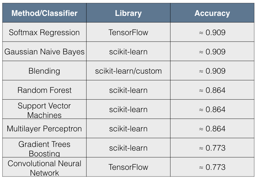
I found the results quite interesting for the following reasons:
- The simpler models such as Softmax Regression and Gaussian Naive Bayes have better accuracy than more complex models.
- The accuracy scores have 3 distinct values across all 8 methods tried.
The immediate conclusion that comes to mind from these results is that there has been overfitting by complex models. Blending, however, seems to be remedying this situation for the 5 scikit-learn classifiers and appears to give a result that is comparable to simpler models.
In terms of performance, it seems that Softmax Regression (also called Multinomial Logistic Regression), which is a discriminative model, is doing as well as Gaussian Naive Bayes, which is a generative model. In fact, this is to be expected since “asymptotically (as the number of training examples grows toward infinity) the GNB and Logistic Regression converge toward identical classifiers”.
However, there is also a famous paper by Profs. Ng and Jordan titled “On Discriminative vs. Generative Classifiers: A comparison of logistic regression and naive Bayes” in which it is argued that given enough data, Logistic Regression will outperform Naive Bayes Classifier.
It seems that non-linear models are doing a poor job in making accurate disease predictions from the microbiome dataset compared to linear models such as Logistic Regression and Gaussian Naive Bayes. Maybe this is a reflection of the microbiome dataset itself rather than the shortcomings of more complex models.
4. Conclusion
In this post, I have tried the application of different machine/deep learning algorithms on a microbiome dataset and assessed the accuracy of each method. It’s not a truly apples-to-apples comparison since different machine learning models have different levels of complexity, work on different assumptions and require different hyper-parameters to tune.
In my opinion, it is, nonetheless, interesting to apply different models on the same dataset in order to learn more about the dataset itself and see if there is any ‘convergence’, so to speak, between the results/performance of different models.
From the perspective of disease diagnosis, our aim is to be as accurate as possible. It is, therefore, worthwhile to apply different models on the data in order to find the one that has highest accuracy. This will ultimately help us in developing a truly powerful diagnostic platform for disease detection and can help in improving the lives of human beings.