Unless otherwise stated, the author asserts his copyright over this file and all files written by him containing links to this copyright declaration under the terms of the copyright laws in force in the country you are reading this work in.
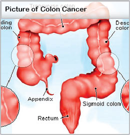
Colorectal cancer is the second leading cause of cancer related deaths in US. The gold standard methods of colorectal cancer detection includes procedures such as colonoscopy and sigmoidoscopy. The problem with procedures such as colonoscopy and sigmoidoscopy is that they are expensive and invasive. There is, therefore, a great need in developing highly sensitive, non-invasive and inexpensive tests to detect colorectal cancer early on.
A number of scientific studies have pointed towards a change in the composition of gut microbiota, as colorectal cancer progresses. This represents an opportunity to explore the development of microbiome-based diagnostics for colorectal cancer detection. Specifically, the microbiome profile of an individual, as obtained from stool sample, can be used a proxy to identify the individuals health status.
In the context of machine learning, we are presented with a supervised learning problem for classification. The microbiome profile for an individual is a vector of OTUs (features). Having a dataset of microbiome profiles of individuals with or without colorectal cancer, we can perform a training-test-split, learn on the training set, perform cross-validation and see how well the predictions do compared to the actual values of the test set.
2. Materials and Methods
A recent study by Baxter et al. published this year in April 2016 demonstrated that random forest classifier did a surprisingly well job at predicting colorectal cancer using microbiome data as input. This was a nice dataset since it had a large number of samples (490) and fewer number of OTUs (335). In this case, p < N. This meant that deep-learning methods would work as well since our feature vector was small (only 335 OTUs) as opposed to the study by Gever et al., which had 9511 OTUs.
Following the approach taken in my previous analyses, I obtained the dataset, which is publicly available on GitHub and compared other supervised learning methods to the random forest classifier used originally in the paper. The analyses I performed differed from the original study in three important ways:
In the original study, there were 3 clinical outcomes: normal, adenoma and cancer. The authors had constructed ROC curves for adenoma vs. normal and for cancer vs. normal. While it is fine to take such an approach, doing this way split of the data reduces sample size for training and testing. Since adenoma is a non-cancerous state, I combined all normal and adenoma samples into a single ‘no-cancer’ category and constructed ROC curves of no-cancer vs. cancer.
In the R code provided with the data on GitHub, it was surprising to note that training-test-split was not performed on the dataset with 490 samples. That is, the random forest classifier was trained and tested on the entire dataset. I did a train-test split.
The authors used R programming language for their analyses and I relied on Python.
The analyses is present on a Jupyter notebook, which can be accessed here.
3. Results
The following ROC curve shows the performance of different classification algorithms in predicting colorectal cancer status
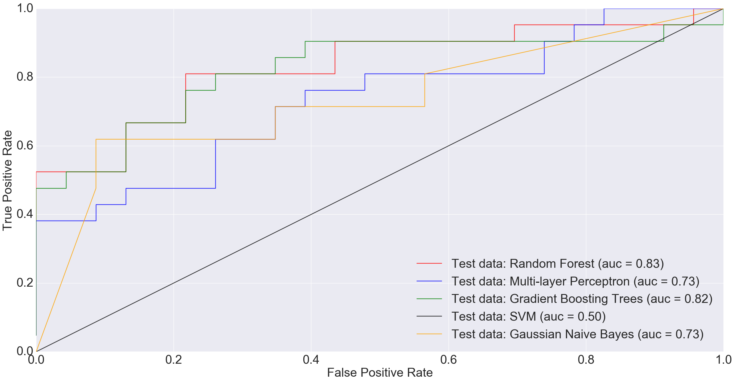
ROC plot comparing the AUC of different algorithms when classifying original non-cancerous vs. cancerous samples (excluding adenomas).
Adenoma was in 198 samples, normal was 172 and cancer was 120. If a binary classification is performed between just the normal samples and cancer samples, our total sample size is 292 (172+120). Doing a 85% training/15% test split i.e., 248 training and 44 test, MLP performed much worse than other models and Random Forest did really well.
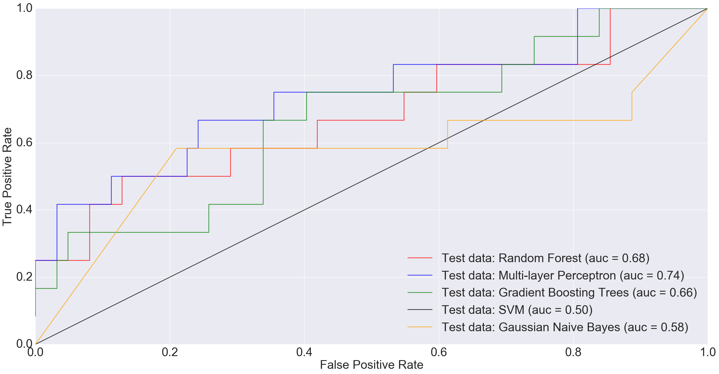
However, at larger sample sizes (416 training and 74 test), when all non-cancerous samples were combined into one group in order to benefit from the entire dataset, MLP performed much better than other models including Random Forest and Gradient Boosting Trees.
ROC plot comparing the AUC of different algorithms when classifying all non-cancerous samples combined (i.e., normal plus adenoma) vs. cancerous samples.
In the plot above, a simple neural net architecture has performed better than more sophisticated algorithms such as Random Forest and Gradient Boosting Trees.
4. Discussion
There is potential in using the microbiota profile as obtained through Next Generation Sequencing (NGS) technologies as proxy for diagnosing difficult diseases. While there is no one best machine learning algorithm out there to do the job, there is great potential in using deep-learning algorithms for this purpose. In future, as datasets grow and algorithms improve, we hope to reach a point where disease detection might routinely rely on machine learning approaches.
5. Acknowledgements
Thanks to Dr. Pat Schloss for pointing towards the study by Baxter et al. and answering some of my questions. Also, thanks to a suggestion by my friend, Ahmet Sinan Yavuz, to try combining all non-cancerous samples into one group before training the models.
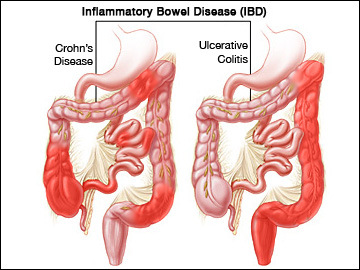
In this post I will be applying machine/deep learning methods to a dataset from one of the largest Inflammatory bowel disease (IBD) microbiome study in humans.
Crohn’s disease and ulcerative colitis: Two types of inflammatory bowel diseases. Image credit: http://nashvillecoloncleansecolonic.com/lower-gi-issues/inflammatory-bowel-disease/
Copyright Declaration
Unless otherwise stated, the author asserts his copyright over this file and all files written by him containing links to this copyright declaration under the terms of the copyright laws in force in the country you are reading this work in.
In my previous posts, I applied different machine learning algorithms to a specific microbiome dataset for HIV prediction. The dataset was quite small and had information of only 51 subjects. The next logical step, in my journey of applied machine-learning for disease detection, was to obtain a larger microbiome dataset.
This I did by getting hold of the files from the study by Gevers et al. The study by Gevers et al. is one of the largest microbiome studies in pediatric inflammatory bowel diseases (IBD) area. Amongst other things, the study explored the role of biopsy-associated microbiome for diagnosis of Crohn’s disease (CD).
The data from this study was obtained from the QIITA website. The OTU table and meta-data file provided information about 1359 human samples, which were divided into 4 categories. 731 subjects had Crohn’s disease (CD), 219 had ulcerative colitis (UC), 73 had indeterminate colitis (IC) and 336 were healthy subjects. The OTU table additionally had information about 9511 OTUs.
To make the classification task simpler, have clear separation between health and disease status and have larger training and test datasets, I combined the UC, IC and CD samples into a single IBD category and kept healthy subjects in their separate category.
Gevers et al. had constructed ROC curves in their original paper to evaluate the performance of sparse logistic regression classier (using L1 penalization) to identify IBD status of subjects based on microbiome profile.
2. Differences from main study
In the analysis I’m posting here, I did three things differently:
Gevers et al. had separated the samples by collection site. To quote from the paper: ‘We included a total of 425 tissue biopsies of the ileum, 300 of the rectum, and 199 stool samples in three independent analyses.’ They had shown three separate ROC curves, each for separate sample type. In the metadata file provided for this study from the QIITA website, there were 641 ileum sample, 309 rectum samples and 283 stool samples. I could not figure out the reason for this discrepancy even after contacting QIITA support team, so I could not get to replicate the analysis by Gevers et al.
It was not clear from the paper whether the authors had pooled together the UC, IC and CD samples together in order to do binary logistic regression or had kept the classes separate and had performed multinomial logistic regression. As stated earlier, I opted for binary classification by grouping all UC, IC and CD samples together.
Gevers et al. only assessed the performance of sparse logistic regression classier (using L1 penalization). In addition to sparse logistic regression classifier with L1 penalty, I also tested the performance of Random Forest, Gradient Boosting Trees, Gaussian Naive Bayes, Support Vector Machine and Multi-layer Perceptron.
All the code for this analysis is present on Jupyter Notebooks hosted on my GitHub and can be seen here and here.
3. Results
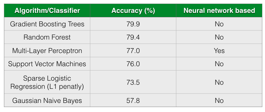
The following table shows the accuracy of different classification algorithms on the dataset by Gevers et al.
Table shows the accuracy of different classifiers. The table is sorted by Accuracy column in descending order.
As seen from the table, all almost classifiers did better than sparse Logistic Regression with L1 penalization except for Gaussian Naive Bayes. Gradient Boosting Trees and Random Forests has almost comparable prediction accuracy followed closely by Multi-Layer Perceptron.
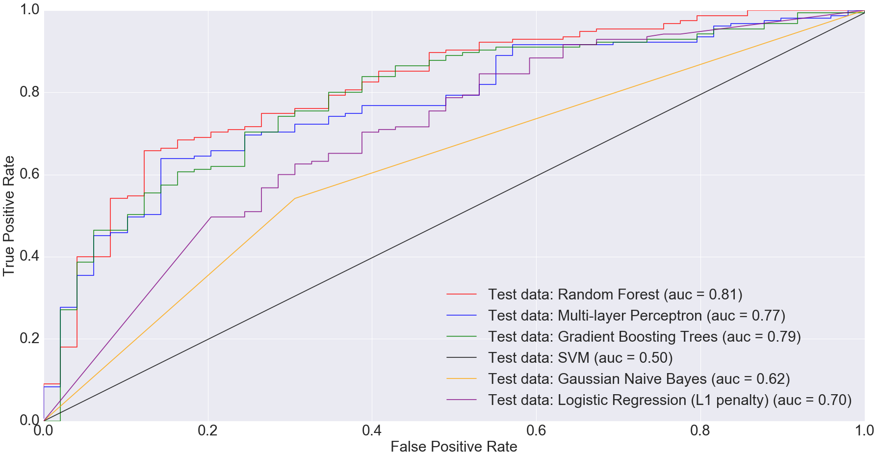
According to Gevers et al., the sparse logistic regression model had second best performance while predicting CD status from rectal biopsies (AUC=0.78). Even though it’s not truly an apples-to-apples comparison, we get comparable AUC with Multi-Layer Perceptron, Gradient Boosting Trees and Random Forest when predicting IBD status from any type of sample (including ileum, rectum and stool). The following figure shows the AUC results.
ROC plot comparing the AUC of different algorithms for all samples
I would argue that my approach is slightly better because we are predicting disease by using different sample types. Ideally, we’d want models that can predict disease status irrespective of sample types. This is important because obtaining certain types of samples such as ileum or rectum biopsies is difficult. Procedures to obtain such samples are invasive and expensive.
Based on the results I’ve shown above, complex models such as random forests and multi-layer perceptron can do a comparable job at predicting disease status irrespective of sample type.
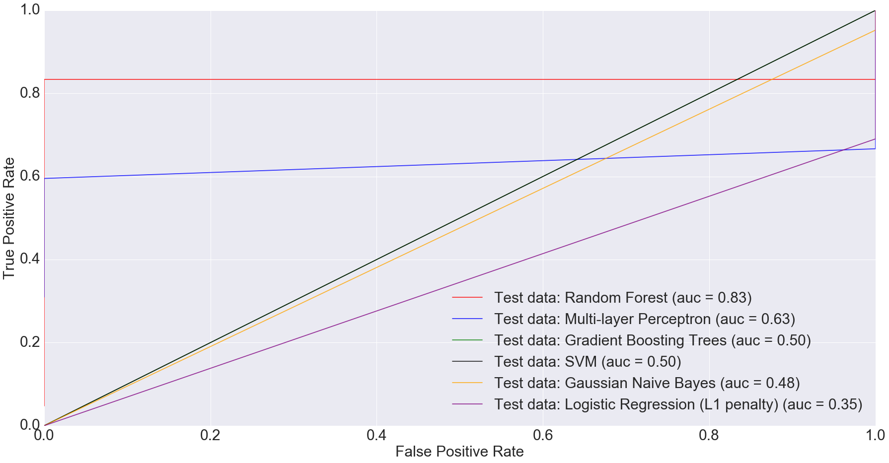
There is also potential in using microbiome data, as obtained from stool samples alone, to do disease diagnosis making the whole process much cheaper and non-invasive. In fact, when we filtered the dataset down to just stool samples (n=283) and trained the models on the smaller dataset, we got some very interesting results. The AUC for logistic regression with L1 penalty was 0.35: the worst among all models.
ROC plot comparing the AUC of different algorithms for only stool samples
Random Forest performed the best with AUC equal to 0.83. The next best performer with Multi-Layer Perceptron with AUC equal to 0.63. This clearly indicates that more complex models have better predictive power when predicting IBD status from stool data, compared to simpler ones.
3A. Convolutional Neural Networks
CNNs, as implemented in TensorFlow, ate all my CPU. I ran the CNN on Gevers et al.’s dataset on my laptop for over 24 hours and it still didn’t finish.
Even though I was successfully able to install GPU enabled TensorFlow on my laptop, I couldn’t get it to work. The following message printed on the terminal screen:
I tensorflow/core/common_runtime/gpu/gpu_device.cc:814] Ignoring gpu device (device: 0, name: GeForce GT 650M, pci bus id: 0000:01:00.0) with Cuda compute capability 3.0. The minimum required Cuda capability is 3.5.
Device mapping: no known devices.
I hope I can get funding and/or collaborative support to access a GPU machine/cluster in order to try convolutional neural networks on the study by Gevers et al. If that happens and I am able to successfully run CNNs on Gevers et al.’s dataset, I will post that as a separate blog entry.
4. Discussion and Conclusion
As seen from this analysis, more sophisticated models have done a much better job at prediction than simpler ones. One of the reasons for this success of complex models over simpler ones probably is large sample size.
Moving forward, I will write a post that will provide some preliminary but promising results on how microbiome plus machine learning beat the state-of-the-art disease diagnosis test for an extremely important disease. Stay tuned!
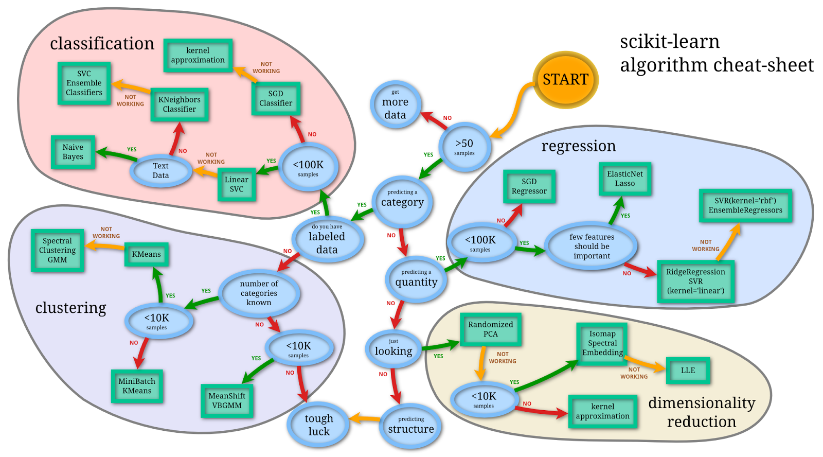
This is a continuation of my previous proof-of-concept posts on applying machine learning algorithms on microbiome data for diagnostic platform development.
Flowchart for finding the right estimator for the job. Image credit: http://scikit-learn.org/stable/tutorial/machine_learning_map/
Copyright Declaration
Except for the image above this declaration, and unless otherwise stated, the author asserts his copyright over this file and all files written by him containing links to this copyright declaration under the terms of the copyright laws in force in the country you are reading this work in.
In order to make medicine truly predictive, we need powerful predictive models that can handle noisy biological datasets. In order to make medicine preventive, we need to detect diseases early on. In this context, disease detection is essentially a problem of classification. Given the input data from an individual, we’d wish to classify the person’s disease status i.e., whether the individual has a disease or not. Once we truly appreciate this fact, we can work towards building better platforms with more sophisticated models that account for the subtleties and stochasticity of biological systems.
Microbiome profile is a proxy for various diseases. Using it as an input, we’d like to know the disease status of an individual. In this post, I will explore the application of some classical machine learning algorithms on microbiome data and see how well they compare to models implemented in TensorFlow that I discussed in my earlier posts, here and here.
This post is a continuation of my previous proof-of-concept posts in which I was using a microbiome dataset as input to deep-learning models in order to predict the HIV status based on a study by Lozupone et al.
2. Technical Details
A number of models exist in machine learning literature that are suitable for classification tasks. Many of these models have different parameters that are not directly learned during the training session. The optimal values of these parameters can be searched in a user-defined parameter search space and subsequently cross-validated.
For this purpose, I ran the GridSearchCV() method with a 3-fold cross-validation on 4 out of the 5 models, which required parameter tuning. I left one model out because it was fairly simple and had no complicated parameters to be searched and cross-validated. The script is called gridsearch.py.
Below are some of the models that I have used in this exploratory analysis that are available in the Python machine learning library, scikit-learn.
2A. Gaussian Naive Bayes
Gaussian Naive Bayes is one of the simplest algorithms used for classification purposes. In this model, the likelihood of the features is assumed to follow a normal distribution. The classifier is called Naive Bayes because it relies on the Bayes theorem to determine the posterior i.e., probability of belonging to a class, given the features. It’s naive in its assumption that all features are independent.
Random Forest classifier is a machine-learning algorithm falling under the category of ensemble learning, which takes the bagging (bootstrap aggergating) approach. Briefly, random forest, as the name suggests, consists of many (random) trees. Each tree is a classifier that is trained independently of other trees.
As a classifier, the tree is developed by randomly selecting a subset of features and performing a split over a number of nodes. The result is the predictions provided by the leaf nodes of the tree. Random forest does this for multiple trees. The final predictions are obtained by averaging over the forest.
[A] natural way to reduce the variance and hence increase the prediction accuracy of a statistical learning method is to take many training sets from the population, build a separate prediction model using each training set, and average the resulting predictions… Of course, this is not practical because we generally do not have access to multiple training sets. Instead, we can bootstrap, by taking repeated samples from the (single) training data set… This is called bagging… The main difference between bagging and random forests is the choice of predictor subset size m. For instance, if a random forest is built using m = p, then this amounts simply to bagging.
Usually, for random forests, the number of predictors considered at each split is approximately equal to the square root of the total number of predictors.
I used the RandomForestClassifier() class from scikit-learn library for prediction. Based on cross-validated grid-search, I used n_estimators = 1000, which is the number of trees and set random_state = 0 as seed for the pseudo random number generator (PRNG).
2C. Gradient Tree Boosting
Like Random Forests, Gradient Tree Boosting classifier is also part of ensemble learning. Unlike Random Forests, it relies on the boosting approach. In boosting, the classifiers are trained sequentially. That is, each new tree is grown utilizing information from trees grown previously. Also, unlike the bootstrapping approach of random forest, in boosting, new decision trees are fit to the residuals of the model. So, instead of fitting the data hard by using a single large decision tree, boosting learns slowly.
The number of trees: Boosting can overfit if number of trees is large.
The shrinkage parameter (λ): This is also called the learn rate and controls the rate at which boosting learns. Small values of λ require large number of trees in order to have good performance.
Number of splits on each tree (d): This is also called maximum depth of the tree and controls the complexity of the boosted ensemble.
I used GradientBoostingClassifier() class with n_estimators=1000, learning_rate=1, max_depth=10 and min_samples_split=5 based on the cross-validated grid-search. The value of random_state was set to 0, which is the seed for PRNG. Rest were default values.
2D. Support Vector Machines (SVMs)
Support Vector Machines (SVMs) are class of supervised learning algorithms that have historically been used for classification purposes. The idea has been to come up with hyper-plane or set of hyper-planes that can separate the samples in two or more classes.
The multi-layer perceptron is a type of artificial neural network that trains using backpropogation. In it’s simplest case, it can be considered as a logistic regression classifier in which the input data is transformed by some non-linear transformation. The intermediate layer with the transformed input is called hidden layer. In a simple network architecture, we can have one hidden layer that can then connected to the output layer by another simple transformation function such as softmax function.
The implementation of MLP in scikit-learn is still in development stages. For this reason, I had to the use the development version of scikit-learn in order to apply this model. At the time of writing, the version is 0.18.dev0.
MLPClassifer() was used with following parameter values based on cross-validated grid-search: algorithm = ‘adam’, alpha = 0.01, max_iter = 500, learning_rate = ‘constant’, hidden_layer_sizes = (400,) and random_state = 0. I additionally set the learning_rate_init parameter to 1e-2 and activation parameter to ‘logistic’. Doing grid search for activation parameter and learning_rate_init ate all my laptop memory, so I manually adjusted them.
2F. Blending
Blending is one of the approaches to create datasets from predictions of different classifiers and then train a new classifier on top of it. I came across this approach while reading a blog entry titled Kaggle Ensembling Guide on MLWave website.
It’s a powerful technique that many top Kagglers use. According to the entry, the advantage of blending is that prevents information leak since generalizers and stackers use different data.
The same blog post referred to a Python script by Emanuele Olivetti, which I modified slightly to read in the microbiome data and perform blending. The generalizers used were the 5 different scikit-learn classifiers: Gaussian Naive Bayes, Random Forests, Gradient Boosting Trees, Support Vector Machines and Multi-layer Perceptron. Final blending was done with LogisticRegression() class of scikit-learn with default values.
All scripts and documentation for the analyses in this and previous posts is available on my GitHub repository called TFMicrobiome.
3. Results
I used the simple score() method for each classifier trained and tested in scikit-learn. According to scikit-learn documentation, the score returns the mean accuracy on the given test data and labels. [It is a] harsh metric since you require for each sample that each label set be correctly predicted.
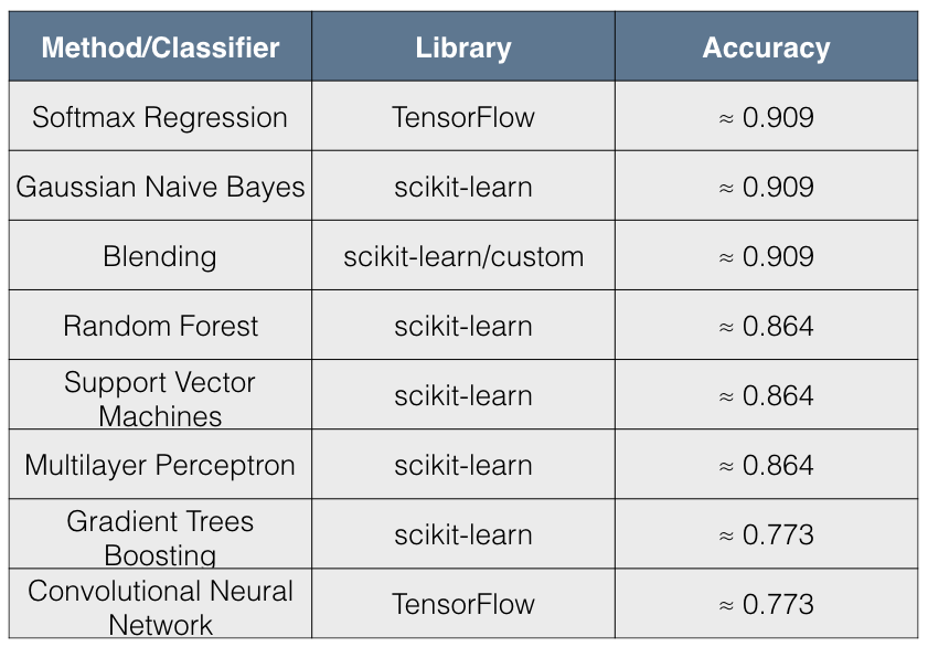
The following table summarizes the results:
Table shows the accuracy of different classifiers. The table is sorted by Accuracy column in descending order.
I found the results quite interesting for the following reasons:
The simpler models such as Softmax Regression and Gaussian Naive Bayes have better accuracy than more complex models.
The accuracy scores have 3 distinct values across all 8 methods tried.
The immediate conclusion that comes to mind from these results is that there has been overfitting by complex models. Blending, however, seems to be remedying this situation for the 5 scikit-learn classifiers and appears to give a result that is comparable to simpler models.
It seems that non-linear models are doing a poor job in making accurate disease predictions from the microbiome dataset compared to linear models such as Logistic Regression and Gaussian Naive Bayes. Maybe this is a reflection of the microbiome dataset itself rather than the shortcomings of more complex models.
4. Conclusion
In this post, I have tried the application of different machine/deep learning algorithms on a microbiome dataset and assessed the accuracy of each method. It’s not a truly apples-to-apples comparison since different machine learning models have different levels of complexity, work on different assumptions and require different hyper-parameters to tune.
In my opinion, it is, nonetheless, interesting to apply different models on the same dataset in order to learn more about the dataset itself and see if there is any ‘convergence’, so to speak, between the results/performance of different models.
From the perspective of disease diagnosis, our aim is to be as accurate as possible. It is, therefore, worthwhile to apply different models on the data in order to find the one that has highest accuracy. This will ultimately help us in developing a truly powerful diagnostic platform for disease detection and can help in improving the lives of human beings.
This is a proof-of-concept post based on the TensorFlow library developed by Google. To the best of my knowledge, it is the first ever attempt to apply Convolutional Neural Networks on microbiome data.
A typical Convolutional Neural Network with convolutional layer, max-pooling and fully-connected layer. Image credit: http://colah.github.io/posts/2014-07-Conv-Nets-Modular/
Copyright Declaration
Except for the image above this declaration, and unless otherwise stated, the author asserts his copyright over this file and all files written by him containing links to this copyright declaration under the terms of the copyright laws in force in the country you are reading this work in.
There is extensive literature on convolutional neural networks (CNN) and it is the beyond the scope of this post to do an extensive survey on CNNs. In this post, I will provide a description of applying CNNs to microbiome data as a proof-of-concept exercise. This is the first time, to the best of my knowledge, that CNNs have been applied to microbiome data. So, without further ado, let’s dive right into CNNs.
2. Technical Details
2A. Reading data
The input file of microbiome data comes as an OTU table. The individual (sample) on which microbiome data is obtained is actually a vector of OTUs. In the Lozupone et al dataset, we have information on 267 OTUs. Our input for CNN, therefore, is a 267x1 vector for each sample.
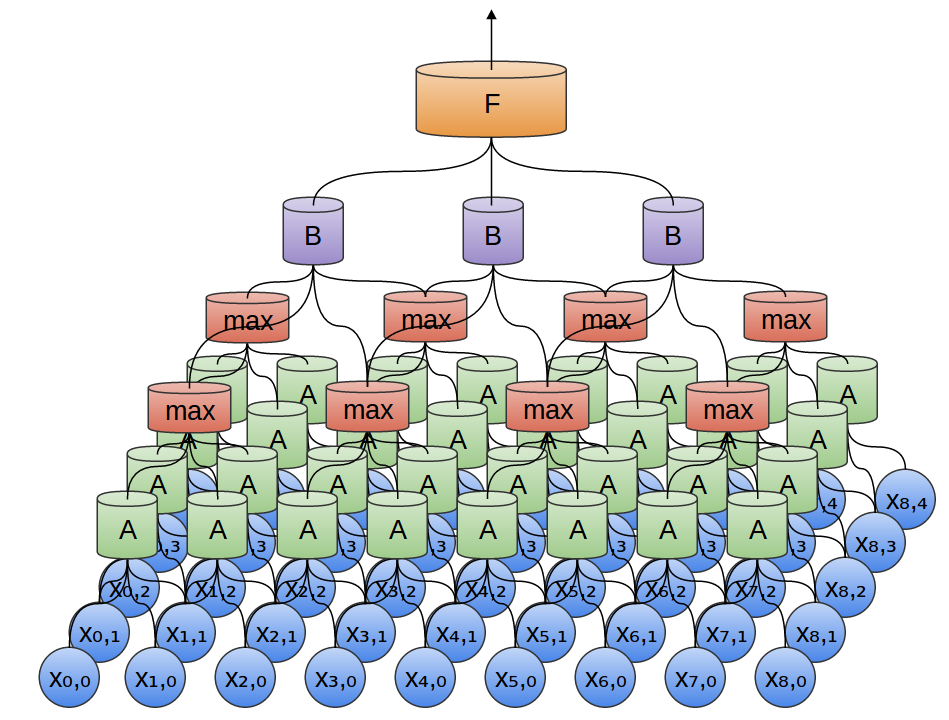
Microbiome input data flow in CNN from bottom to top.
To elaborate the figure a bit more:
The OTU table is input for the first convolutional layer followed by max-pooling.
The output of first max-pooling is input to second convolutional layer followed by max-pooling.
The output of second max-pooling is input to densely connected layer.
Dropout is performed on the output of densely connected layer.
The output of dropout is finally passed to the readout layer, which performs simple softmax regression.
2C. Input reshaping
In traditional image classification datasets, such as MNIST, one would like to reshape the flattened image pixel vector back to the original 2d image array.
tf.nn.conv2d method in TensorFlow library, which computes a 2-D convolution given 4-D input and filter tensors can be used for this purpose. Unlike the MNIST dataset, in which the in_height and in_width of the input tensor can be set to 28x28, in the microbiome dataset, the in_height and in_width are set to 1 and 267 respectively, where 267 is the number of OTUs (features) in the dataset.
3. Results
Even though CNN model is more sophisticated than basic softmax regression, we get a much lower accuracy (of about 0.772) for our dataset using CNN. I have tried playing around with different variables and parameters. Following are some of the variables I have tried to manipulate.
Train-to-test split ratio: The highest accuracy I got was with train to test ratio of 0.55.
Max-pooling: Whether one does max-pooling or not, it did not seem to have an impact on accuracy with the current microbiome dataset.
Dropout: Like max-pooling, doing or not doing dropout does not seem to be impacting the accuracy.
Gradient descent optimizers: AdadeltaOptimizer with learning_rate = 0.1, rho = 0.95 and epsilon = 1e-02 seems to be giving accuracy of 0.77. I have also tried AdamOptimizer and it seems to be giving comparable results. I haven’t tried other optimizers.
Stride for conv2d and maxpool: The highest accuracy is when the stride of the sliding window is 1 for both conv2d and maxpool at the start of the script i.e., the input to the first convolutional layer.
Changing activation functions: Changing the activation functions from relu to relu6, elu, sigmoid, tanh, softplus and softsign didn’t change the accuracy.
Bias variable initialization: I changed the value of bias variable initialization from 0.1 to 1 to 10 to 100 but did not see increase in accuracy.
Few variables that I have not explored so far include:
Changing the number of convolutional layers
Changing the output channel values of convolutional layers
Randomizing the training and test datasets
4. Discussion
One reason for the relatively poor performance of convolutional neural networks over softmax regression, maybe, has to do with the type of input data. CNNs are great for tasks such as image classification because they can take into account the spatial structure of the data. In image classification, for example, input pixels which are spatially closer together would have higher correlation than pixels far apart.
In the microbiome dataset, however, there is no corresponding spatially local correlation that CNNs can exploit by enforcing a local connectivity pattern. One way to develop an analog for spatially local correlations in microbiome data is to utilize the phylogenetic relationship information between OTUs. That is, OTUs that are evolutionarily closer can have higher correlation than OTUs that are evolutionarily distant. This is something I can explore in future posts.
Summing up, even though CNN has not done a better job compared to basic softmax regression, there is potential for further fine tuning this model. Larger microbiome datasets can be used for this purpose, evolutionary information can be taken into account and further parameter tuning can be done in order to improve the predictive power of the model.
This is a proof-of-concept post based on the TensorFlow library developed by Google. The idea is simple: using a publicly available microbiome dataset, I wish to apply deep-learning algorithms for potential diagnostic platform development.
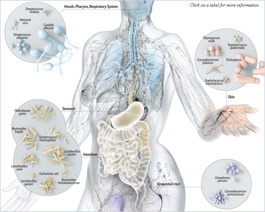
Distribution of different bacteria in different parts of the body. Image credit: http://www.bioxplorer.com/human-microbiome/
Copyright Declaration
Except for the image above this declaration, and unless otherwise stated, the author asserts his copyright over this file and all files written by him containing links to this copyright declaration under the terms of the copyright laws in force in the country you are reading this work in.
There is great potential for growth in and capitalization of the microbiome market. Large companies such as DuPont, JNJ and Merck along with small startups such as Second Genome, Whole Biome, Phylagen and ubiome, to name a few, are catering to this market.
Microbiome-based diagnostics
The composition of our microbiomes has been shown to be correlated with numerous disease states by growing amount of scientific literature. The human microbiome, therefore, has an important role in the diagnosis and early detection of various diseases.
Microbiome data can be leveraged to achieve one of the goals of systems biology in making medicine predictive, preventive, personalized and participatory. This is known as P4 medicine.
In the following sections, I have developed a simple deep-learning model using the microbiome data to predict the HIV status of individuals based on a simple Softmax Regression model.
Technical Details
Data collection
For the purpose of demonstration, I will focus on a single study carried out by Lozupone et al. The study by Lozupone et al showed an association of the gut microbiome with HIV-1 infection. Using this knowledge, I obtained the dataset for this study, which is made publicly available by the Qiita microbiome data storage platform.
The dataset obtained from Qiita for Lozupone’s study had HIV-1 status information available for 51 individuals. 30 individuals are HIV-1 positive and 21 individuals are HIV-1 negative.
Model building
Given the limited human and computational resources I had access to i.e., myself and my laptop, I built a fairly simplistic softmax-based regression model.
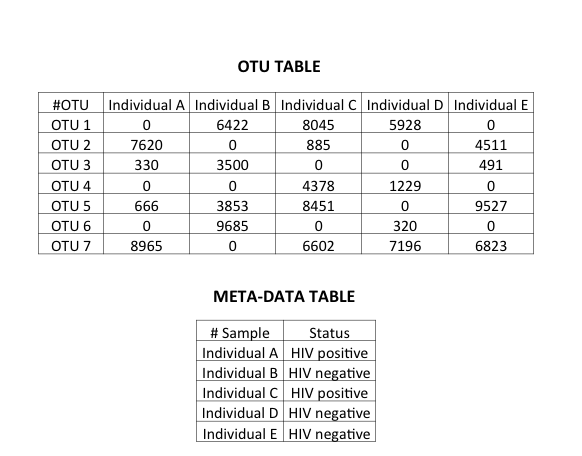
A microbiome dataset consists of a count matrix in which the bacteria characterized by Next Generation Sequencing (NGS) are the rows and the samples from which the bacterial count information is obtained are columns. Additionally, there is meta-data associated with the samples. On a technical note, the bacterial count here refers to OTUs.
Microbiome data: An OTU table with random OTU counts and a meta-data table providing additional information about samples included such as disease status.
It is beyond the scope of this post to go into the definition of OTUs. Suffice to say, I am treating bacteria/OTUs as input features in the model. On a related note, OTU tables are sparse matrices.
The response variable is the disease state. In this particular dataset, it is the status of HIV-1, which is either positive or negative. The dataset had information about 267 bacteria/OTUs i.e., features. The training set had 29 samples and testing set had 22 samples.
Model evaluation
Using the input data for Lozupone’s study, I wrote a simple Python script that ran softmax-regression. The script and further technical specs are on my GitHub repository called TFMicrobiome.
Even though the dataset was small and the model simple, I ended up getting an accuracy of 91%! This demonstrates that even the most simplistic of deep-learning system is very powerful in dealing with real-life noisy data and has the potential to be developed into a diagnostic platform.
Future Directions
Moving forward, there are three broad areas where effort needs to be put in.
Other biological datasets
I have made use of only a small microbiome dataset. From a statistical perspective, the sample size is small and there is a need for larger datasets to train the models.
Additionally, and from a biological point-of-view, microbiome is part of the picture. At a molecular level, there are other high-throughput datasets available such as that of the genome, transcriptome, proteome and metabolome. By integrating the various ‘omics’ datasets for a given individual, we can develop a truly systems level understanding of various biological diseases and achieve the objectives of P4 medicine.
Other deep learning algorithms
As a simple POC, I made use of the simplistic softmax regression model. It is not the most powerful method out there. Moving forward, I’d like to see some more sophisticated algorithms being employed such as convolutional neural networks and recurrant neural networks, to name a few.
Feature selection in deep-learning
One of the aims of medicine is to make inference. That is, given the diagnosis, how can one know etiology of the disease and develop appropriate intervention and prevention strategies. In the context of deep-learning for microbiome, the aim is not just to make a prediction about disease. It is also about feature selection. We’d like to know which features i.e., microbes, are important in causing or preventing the disease. This will help in the development of therapeutics.
The challenge, therefore, is to develop a deep-learning system that can, apart from making accurate prediction about diseases, can also provide information of about the microbes, genes, proteins and metabolites that impact the health status.